Processing Steps
- Quality Control & standardization
What We Did. We removed non-earthquake entries (e.g., quarry blasts), coerced key fields to valid types, and normalized timestamps to UTC. Invalid coordinates and implausible magnitudes were dropped, duplicate event IDs were de-duplicated, and the catalog was stably sorted in time. Because the raw feed mixes magnitude scales, we standardized all magnitudes to moment magnitude (Mw) for analysis: Mw/Mwr/Mh were kept as-is; ML/MLr, Mb, Ms, and Md/Mc were converted to Mw using conservative linear mappings with explicit validity ranges; unrecognized or low-quality types (Ma/Fa/Mfa/"uk") and out-of-range values were excluded. We then applied a working floor of Mw ≥ 3.0 to align with completeness.
Key findings. Sharp increases in measured seismic events in both the 1930s and 1970s corresponding to advancements in seismic measuring technology. The 1933 Long Beach earthquake sparked the creation of a network of integrated seismometers in the state. The network was expanded again in the 1970s following the 1971 San Fernando earthquakes. Concurrent with these expansions were the development of two seismic measurement scales, both at Caltech: the Richter scale in 1935 and the Moment Magnitude scale in the late 1970s.
- Declustering
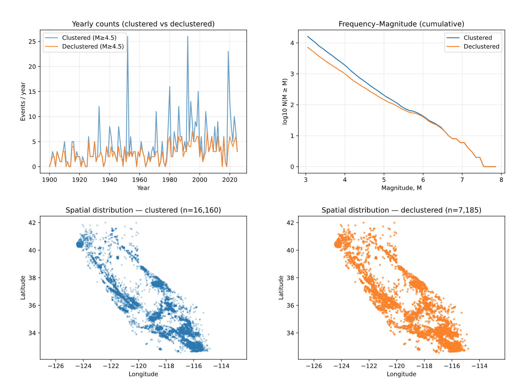
We applied the Gardner–Knopoff (1974) declustering to separate dependent seismicity (foreshocks, aftershocks, swarms) from independent mainshocks. GK uses magnitude-dependent time and distance windows: larger events cast longer and wider “influence” windows, within which smaller events are treated as dependents of the mainshock. We interpolated a standard GK lookup table to obtain a continuous window function and added conservative minimum floors for time and radius.
Implementation. After time-sorting the catalog, we performed a forward sweep: for each candidate mainshock, we flagged subsequent events that occurred within its GK time window and within the great-circle haversine radius, provided they were not larger than the mainshock (with a small magnitude wiggle allowance). Each mainshock spawned a stable cluster_id, and dependents inherited that cluster while also recording a parent_id. We followed with a backward look-back sweep so potential foreshocks just prior to a mainshock, but inside the same GK window, were also assigned—reducing sequence fragmentation.
Sequence consolidation. We built cluster representatives (maximum-magnitude event per cluster) and used a union–find merge step: representatives were merged only when their time windows mutually overlapped and their epicenters were closer than a strict fraction of the smaller GK radius. This dual gate (time ∩ space) prevents accidental merges while consolidating genuine multi-burst sequences.
Controls & outputs. The procedure is fully parameterized—time/radius scale factors, minimum window floors, merge-distance fraction, and magnitude wiggle—so sensitivity checks are straightforward. We output a clustered catalog (all events with cluster_id, parent_id, is_mainshock) and a declustered catalog (mainshocks only), alongside simple sanity summaries to confirm expected behavior. Overall, the approach is conservative, reproducible, and aligned with standard practice for preparing catalogs for rate and Gutenberg–Richter analyses.
Key findings. Major California sequences appear as spikes: 1933 Long Beach, 1952 Kern County, 1971 San Fernando, 1980 Mammoth Lakes, 1983 Coalinga, 1986 Chalfont Valley Series, 1989 Loma Prieta, 1992 Landers/Big Bear, 1994 Northridge, 1999 Hector Mine, 2003 San Simeon, and 2019 Ridgecrest.
- Completeness
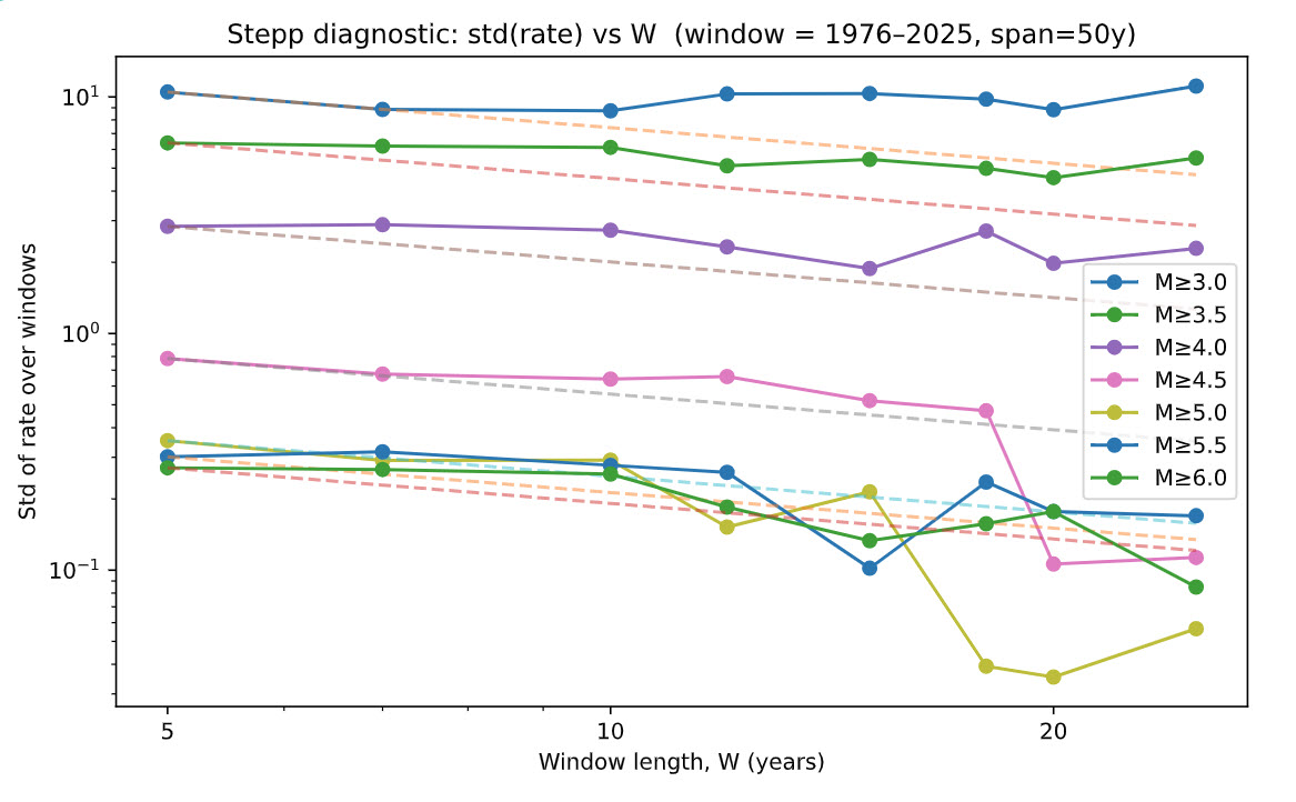
We used a Stepp-style diagnostic to identify the time scale over which the declustered catalog behaves as a stationary Poisson process and to determine a defensible magnitude of completenessMc. The method examines how the variability of annual rates decays with increasing averaging window length W; for a stable, complete catalog the standard deviation of the rate should decrease approximately as 1/√W.
Implementation. We fixed an analysis window by year (toggle SPAN_YEARS = 50/75/100, optionally pinned by END_YEAR_MANUAL) and computed yearly event counts for several magnitude thresholds (e.g., 3.0–6.0). For each threshold, we built non-overlapping windows of length W from a span-aware candidate set (e.g., 5, 7, 10, …, 50 years). Within each W, we aggregated counts to rates and computed the cross-window standard deviation. We plotted std(rate) vs W on a log–log scale with a dashed 1/√W guide to reveal the “elbow” where short-term noise and incompleteness give way to stable behavior.
Completeness (Stepp) selection. Using the declustered catalog, we analyze a fixed calendar window controlled by SPAN_YEARS (optionally anchored with END_YEAR_MANUAL). For each magnitude threshold, we: (1) build yearly counts within the span, (2) compute rate variability over a set of feasible, non-overlapping window sizes WINDOW_SIZES (years), and (3) search for the earliest start year whose fixed-width-bin coefficient of variation (CV over BIN_SIZE_YEARS) stays below CV_THRESHOLD for at least MIN_SPAN_YEARS, with a minimal event-count guard. The per-threshold start years are then consolidated into a piecewise time series of completeness, Mc , by taking the smallest threshold active at each start boundary.
Notes & safeguards. We work on a declustered catalog to limit aftershock bias, use non-overlapping bins to reduce serial correlation, and recompute WINDOW_SIZES whenever the span changes. On the Stepp plot, adherence to the 1/√W trend is a visual check of steady Poisson-like behavior; systematic excess variance at short windows flags incompleteness. The resulting Mc segments form the audit trail for Gutenberg–Richter fitting and rate estimation.
Key findings. The "Stepp step" coupled with the Gutenberg-Richter fitting were the most user-intensive in the analysis. After toggling at varying time windows and minimum Mc thresholds, the 50-year window with Mc=3.0 was determined as the best fit for the model. The 50-year window was chosen due to the known measurement shift in the 1970s as well as to capture two significant earthquakes, Loma Prieta in 1989 and and Northridge in 1994.
The Stepp Analysis below proved difficult to interpret given the inconsistencies between the 'top' and 'bottom' magnitudes, and consideration was given on how much credibility it should be applied in determining proper window and minimum threshold. In researching interpretations of Stepp Analysis, the original typewritten paper can be found with the following underlined statement "For each intensity class, the interval must be long enough to establish a stable mean rate of occurrence and short enough that it does not include intervals in which the data are incompletely reported. This amounts, in practice to minimizing the error of estimate in the mean rate of occurrence of each earthquake class." Given the original intent of the analysis, we confirm the choice in the 50-year window.
- Gutenberg-Richter Fitting
We estimate G–R parameters on the declustered, completeness-filtered catalog within a fixed, recent window. The objective is a defensible magnitude–frequency model where b controls the small/large event balance and a sets overall productivity.
Preparation. Using the Stepp-derived completeness segments, we keep only events with M≥Mc(t) , then restrict to a reproducible LOOKBACK_YEARS window (50 years in this run). We build the frequency–magnitude distribution (FMD) at a fixed bin_width (0.1), computing both incremental counts and cumulative counts N(M ≥ m).
Lower bound and model family. The fit is performed on a stable tail above Mmin (respecting the Stepp floor; here Mmin=3.0). We compare:
- Single-slope GR (one line in log10N vs. M).
- Two-slope GR with an unknown break magnitude Mb(piecewise linear in log10N vs. M, continuous at the break).
Estimation & selection. For any chosen lower bound (and candidate break, if piecewise), we use the Aki–Utsu MLE for b with a binning correction:bMLE = log10(e) / (mean(M) − (Mmin − Δ/2)), then aMLE = log10 N(M ≥ Mmin) + b · Mmin, and σb ≈ b/√N. We grid-search Mb and select the model by AICc. OLS on the cumulative FMD is retained as a QC overlay only.
Anchoring for simulation. To carry realism into the Monte Carlo, we “SIM-anchor” the piecewise model so its predicted N(M ≥ 4.0) exactly matches the observed rate in the fitting window. This preserves mid-magnitude productivity while still honoring the selected slopes above and below the break.
Notes & safeguards. We fit only above completeness, enforce continuity at the break, report AICc for model choice, and publish observed-vs-predicted tables for transparency. The resulting parameters feed the stochastic event generator and all downstream hazard calculations.
Key findings. Selecting a broad enough time window and adequate minimum magnitude while also passing a Kolmogorov-Smirnov test proved challenging. After consideration and interpretation of the Frequency-Magnitude fit, we determined a two-slope model would better fit the data. The magnitude 4.3 was selected as it was high enough to best capture the split and low enough for proper event credibility. Some noise still remains at the higher magnitudes but such is to be expected when managing low frequency data.
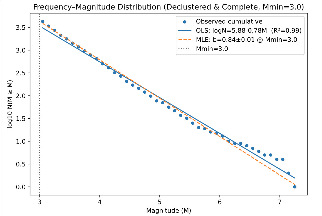
Magnitude–frequency (log10 N–M) with Gutenberg–Richter fit; straight line indicates b-value.
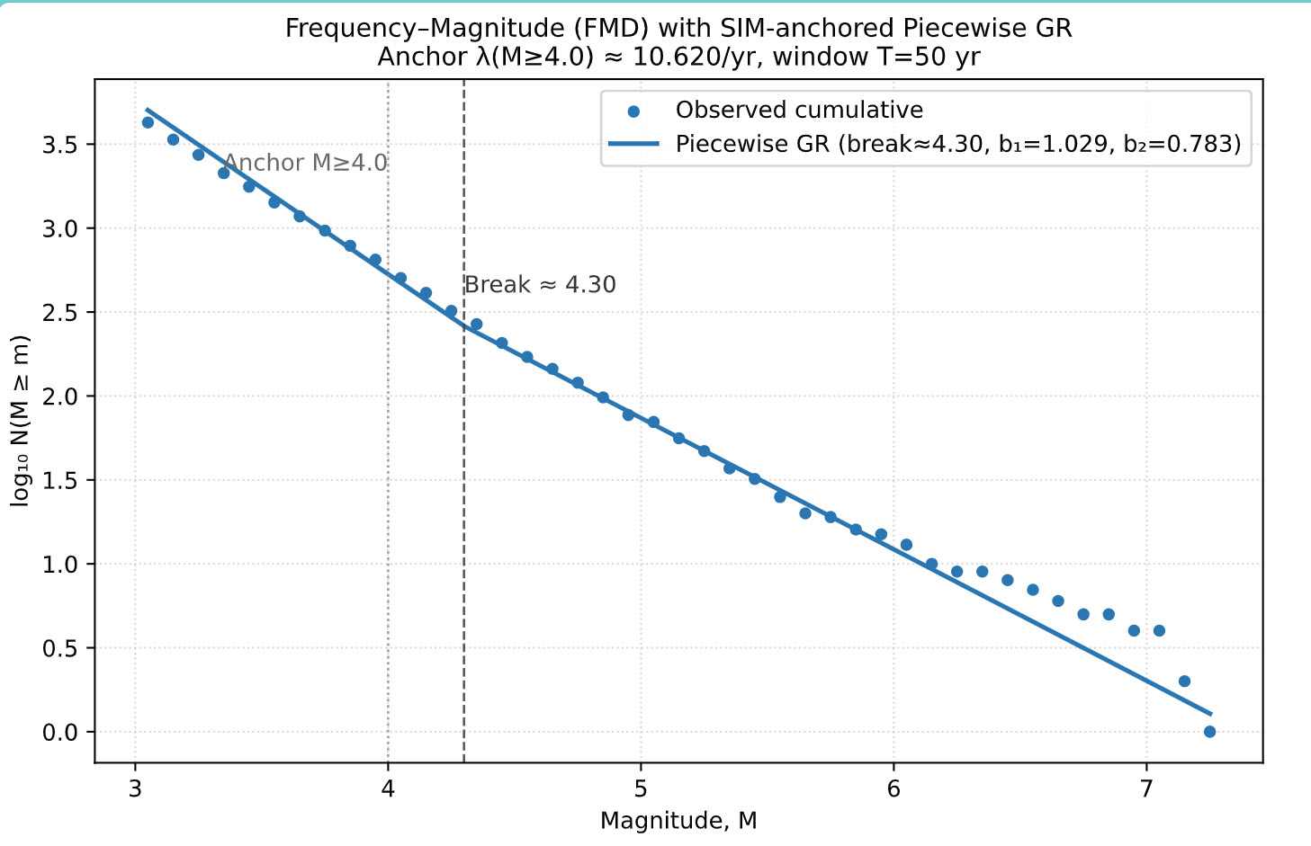 Magnitude–frequency (log10 N–M) with two-slope Gutenberg–Richter fit; straight lines indicate b-values.
- Hazard Grid and Site Data
This module synthesizes a teaching exposure, maps assets to a reusable hazard grid, and attaches site-condition metrics (Vs30) both at asset locations and at grid centroids. The workflow is parameterized, auditable, and saves intermediate artifacts for reuse.
1) Exposure synthesis (locations & attributes)
We load a California state polygon in WGS84 and sample asset coordinates with a metro-weighted strategy plus a uniform rural tail. Metro points are drawn by Gaussian jitter around named metro centers with safeguards to ensure points fall inside the California polygon; rural points are sampled uniformly within the state outline.
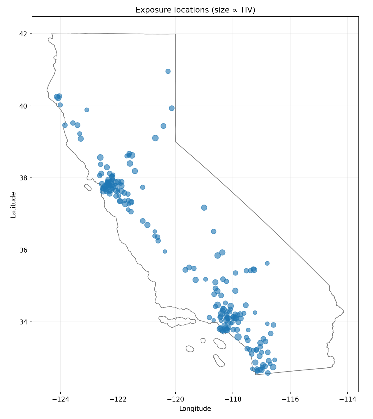 Synthetic exposure: metro-biased sampling with a statewide rural tail.
2) Hazard grid construction & asset mapping
We build a regular lon/lat grid over the California bounding box using a configurable spacing D (degrees). Each grid cell stores its polygon and centroid (lon_c, lat_c). Assets are assigned to the cell thatcontains them via a spatial join; assets outside the grid’s bounding box use anearest-cell fallback to guarantee a mapping.
3) Vs30 sampling at asset locations
We read a Vs30 raster (vs30_slope.tif) and sample values at each asset location. Coordinates are transformed to the raster CRS as needed. We use a bilinear VRT to obtain smooth values and treat raster nodata as NaN. Any nodata or out-of-bounds points are re-sampled with a nearest-neighbor VRT as a targeted fallback. Final values are clamped to a plausible range and remaining invalids are set to a neutral default.
4) Vs30 at grid centroids (for hazard caching)
To support hazard precomputation, we also sample Vs30 at each grid cell’s centroid using the same bilinear-then-nearest procedure. This creates a reusable site-condition layer for the grid, avoiding per-run raster I/O during hazard evaluation.
Reproducibility & tuning
Random seed
Exposure sampling uses a fixed RNG seed for reproducible layouts.
Metro mix
Adjust weights and jitter to emphasize/relax urban concentration; rural share keeps statewide coverage.
Grid resolution
D trades accuracy for performance; finer grids increase file size and join costs.
Raster sampling
Bilinear for smooth Vs30; nearest only for nodata/out-of-bounds recovery.
Together, these steps yield a consistent hand-off from catalog curation to hazard and loss modeling: assets are geolocated, binned into grid cells, and enriched with Vs30 both at the asset and grid levels for fast, repeatable downstream computations.
Hazard
We simulate earthquake events from the fitted Gutenberg–Richter model and compute site-specific shaking using an OpenQuake GMPE. The pipeline supports finite-fault geometry for large events, realistic aleatory variability (between/within), spatial correlation, and produces per-asset intensity measures for downstream loss modeling.
Inputs
- GR source model:piecewise G–R (selected) with SIM-anchored rate (e.g., λ(M≥4.0)).
- Exposure: asset table with asset_id, lon, lat, Vs30, stories/year built (for per-building period).
- Site grid: grid.geojson with centroid Vs30 for caching.
Event sampling
- Counts & timing: number of events ~ Poisson(λ × SIM_YEARS); each event gets a sim_year and a fractional time-in-year.
- Magnitudes: inverse-CDF draws from truncated GR using the selected piecewise fit.
- Locations: epicenters sampled from the declustered catalog’s spatial pool with small jitter (preserves regional patterns).
Finite-fault geometry (large events)
For M ≥ FF_MIN_MAG, we replace point sources with a rectangular planar fault: length/width follow Wells–Coppersmith-type scaling; strike is sampled around a CA-typical NW–SE trend; dip and top-of-rupture (ztor) follow shallow strike-slip heuristics and are capped by a seismogenic thickness. We then compute OpenQuake distances (Rjb, Rrup, Rx). Smaller events use a point-source fallback with depth/rake defaults.
Ground-motion model
- GMPE: Boore et al. (2014, NGA-West2) via OpenQuake (BooreEtAl2014).
- Site context: Vs30 per asset; Z1.0 left undefined when not available.
- Aleatory variability: for each event, draw a between-event term η (~N(0,1)); for each site, draw a within-event vector ε. Optionally apply an exponential spatial correlation to ε with range CORR_RANGE_KM; otherwise i.i.d.
- IMs produced: PGA, SA(0.3 s), SA(1.0 s), and a per-building period SA(T1) by binning each asset’s proxy period to a small set of periods. MMI is derived from PGA for communication./li>
Deterministic ShakeMap add-on
Four selected historical/what-if scenarios for Northridge, Loma Prieta, Landers, and Ridgecrest are included by sampling USGS ShakeMap rasters (MMI/PGA) at asset points. We use GDAL’s WarpedVRT for safe on-the-fly reprojection (bilinear with a nearest fallback) and convert between MMI↔PGA as needed.
Safeguards & QA
- Distances and GMPE contexts follow OpenQuake APIs; all arrays are consistently shaped.
- Event rates are anchored to the selected GR model (SIM-anchored) to match observed λ(M≥4.0).
- Finite-fault width is limited to avoid penetrating below the seismogenic cap; point sources use a sane depth.
- Chunked I/O for large runs; Parquet with CSV fallback; schema stable across simulation and scenarios.
- Residuals module (next section) can be run on the same outputs to verify η/ε distributions and QQ plots against Normal(0,1).
This hazard stage produces the auditable, per-asset shaking dataset that drives the vulnerability/financial layers—while remaining flexible (finite faults, spatial correlation, ShakeMaps) and reproducible via explicit controls and saved artifacts.
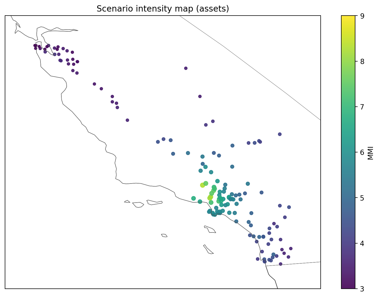
Example ShakeMap of the 1994 Northridge earthquake displaying ground shaking intensity at our portfolio asset locations (marker size/color scale with IM).
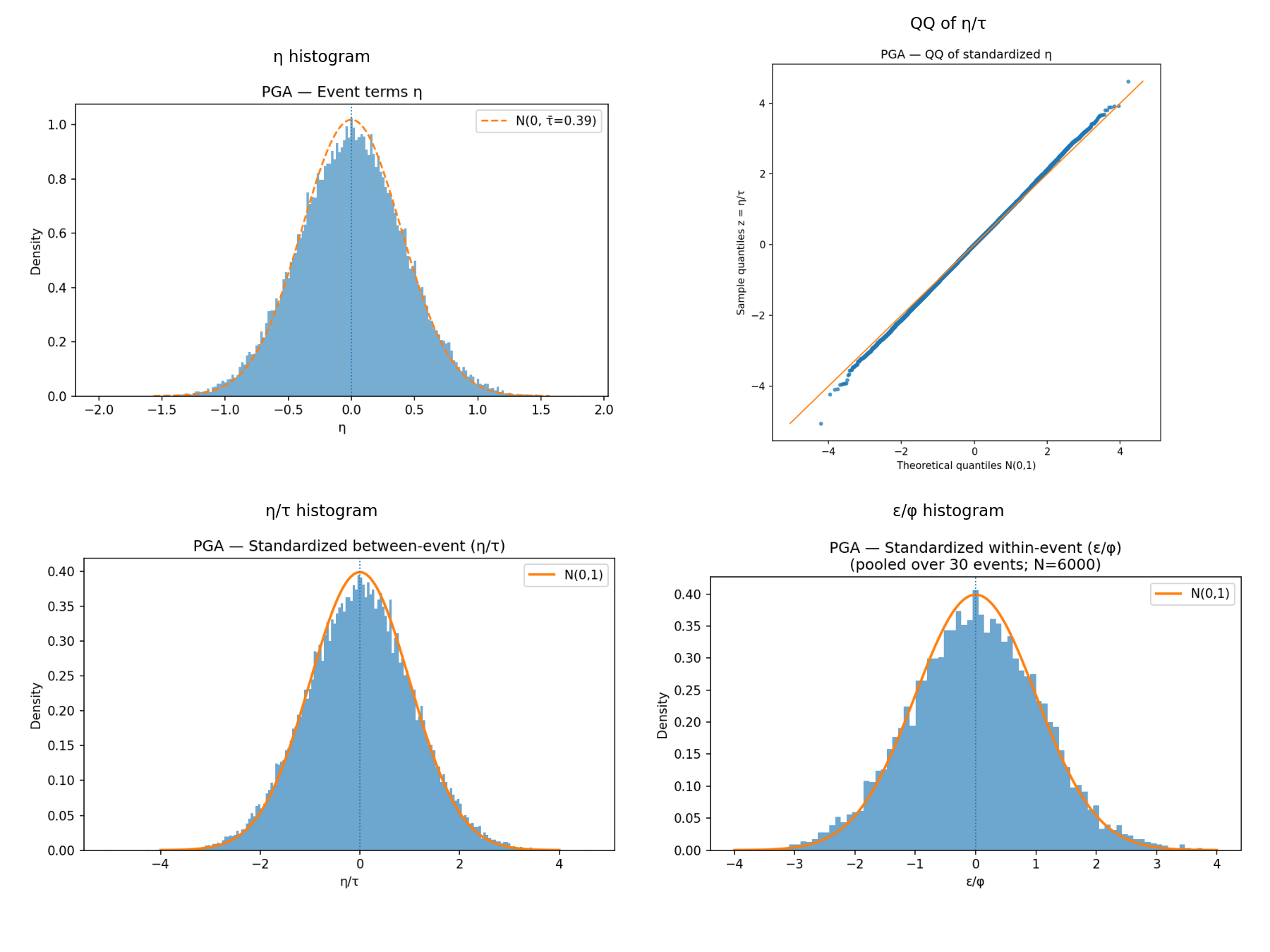
GMPE residuals split into within‑ and between‑event components; QQ panel checks normality.
Vulnerability
This stage converts per-asset ground motions into damage and monetary loss. We use auditable vulnerability curves driven by spectral acceleration at each building’s period (SA(T1)), apply secondary uncertainty (with optional spatial correlation), and stream results to disk for large simulations.
Inputs
- Hazard IMs: per-asset intensities from the Hazard module (SA_T1_g, SA1p0_g, SA0p3_g, PGA_g, MMI).</li>
- Exposure: asset_id, TIV, occupancy, year_built, coordinates./li>
- Curves: occupancy-keyed parameters saved to vuln_used.json.
Damage model
For each occupancy, the mean damage ratio (MDR) is a capped logistic in log-IM:
MDRmean(SA) = cap × σ(a + b × ln(SA + s0))
- a, b, cap, s0 come from the selected curve.
- Driver IM: SA_T1_g by default (falls back to PGA_g if unavailable).
- Era adjustments: coefficients/caps shift by build era (pre-1970, 1970–1994, 1995–2009, ≥2010).
Secondary uncertainty
We sample a lognormal factor with mean 1: exp(σ_SU·z − 0.5·σ_SU²), where z ~ N(0,1). σSU is curve- and era-dependent.
- Spatial correlation: event-wise correlated z across assets with R(d)=exp(−d/CORR_RANGE_KM); otherwise i.i.d.
Loss calculation
- Gross loss: loss_gross = MDR_sampled × TIV per (event, asset).
- Provenance: IMs and metadata (source, scenario_name) are passed through for QA.
Safeguards & QA
- MDR clipped to [0, cap]; losses to [0, TIV].
- NaN/typing checks on TIV and IMs; informative errors on missing columns.
- Era shifts/caps bounded to avoid unrealistic jumps.
- Correlation falls back to i.i.d. if the covariance isn’t PD.
Result: a transparent loss engine that honors building-period effects, uncertainty (including spatial correlation), and portfolio heterogeneity—yielding per-event, per-asset losses ready for financial terms and risk aggregation.
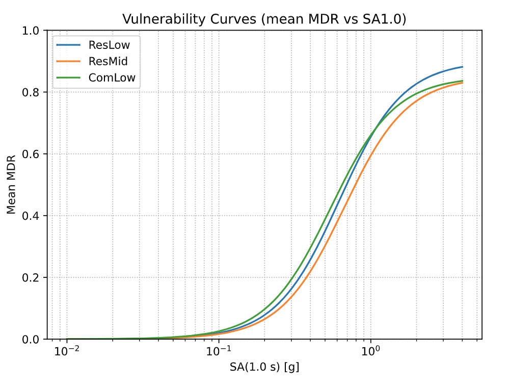
Asset Vulnerability Curve
Financial Terms
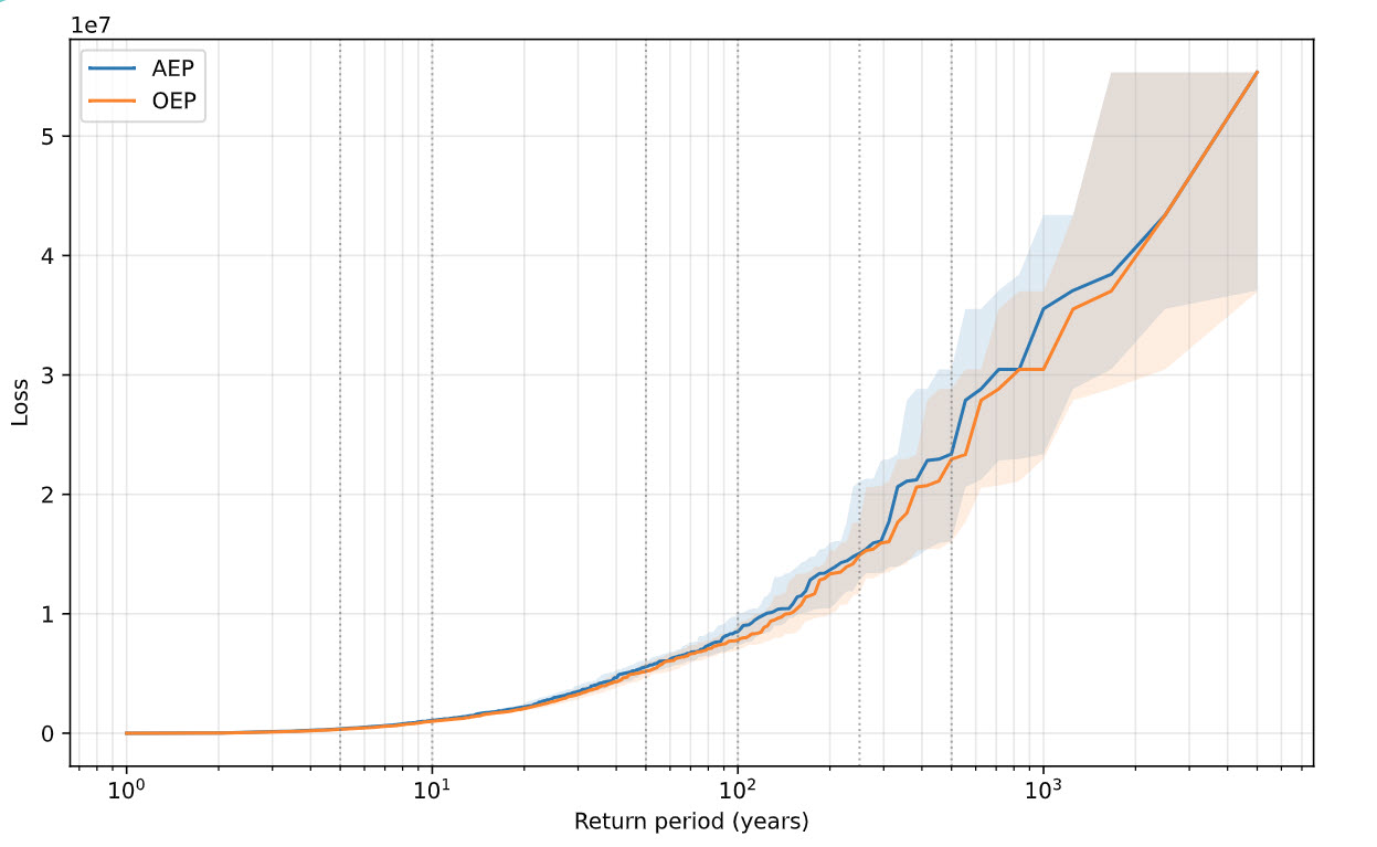
In our final module , we turn per-asset gross losses from the Vulnerability stage into financial losses by applying per-risk occurrence terms (deductibles, limits, optional per-occurrence caps), then rolls them up to per-event totals. As a result, per‑risk deductibles and occurrence limits compress small/medium losses while preserving the tail. We compare Gross vs Net PML (OEP) at standard return periods to make the effect concrete.
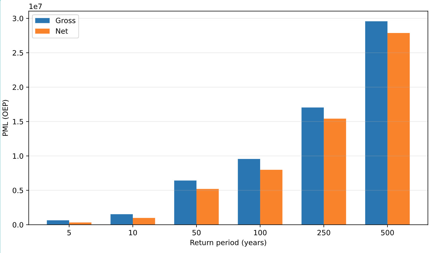
Gross vs Net PML (OEP) at 5/10/50/100/250/500 years.
Results
|